Smoothing function with a bisquare kernel or median.
(Fonction de lissage à partir d'un noyau bisquare ou de la médiane.)
Usage
btb_smooth(
  pts,
  sEPSG = NA,
  iCellSize = NA,
  iBandwidth,
  vQuantiles = NULL,
  dfCentroids = NULL,
  iNeighbor = NULL,
  inspire = FALSE,
  iNbObsMin = 250
)
Arguments
- pts
A
data.framewith cartesian geographical coordinates and variables to smooth. (x, y, var1, var2, ...)(Un
data.framecomportant les coordonnées géographiques cartésiennes (x,y), ainsi que les variables que l'on souhaite lisser. (x, y, var1, var2, ...)- sEPSG
EPSG code of projection (
character). For example, the RGF93 / Lambert-93 projection has "2154" code.(code EPSG de la projection (
character). Par exemple, la projection RGF93 / Lambert-93 a pour code "2154".)`- iCellSize
Cell size of the grid (
integer). The unit of measurement is free. It must be the same as the unit ofiBandwidthvariable.(Taille des carreaux (
integer). Le choix de l'unité de mesure est laissé libre à l'utilisateur. Elle doit seulement être la même que celle de la variableiBandwidth.)- iBandwidth
Radius of the Kernel Density Estimator (
integer). This bandwidth acts as a smoothing parameter, controlling the balance between bias and variance. A large bandwidth leads to a very smooth (i.e. high-bias) density distribution. A small bandwidth leads to an unsmooth (i.e. high-variance) density distribution. The unit of measurement is free. It must be the same as the unit ofiCellSizevariable.(Rayon de lissage de l'estimation d'intensité par noyau (
integer). Cette bande-passante se comporte comme un paramètre de lissage, controlant l'équilibre entre biais et variance. Un rayon élevé conduit à une densité tres lissée, avec un biais élevé. Un petit rayon génère une densité peu lissée avec une forte variance. Le choix de l'unité de mesure est laissé libre à l'utilisateur. Elle doit seulement être la même que celle de la variableiCellSize.- vQuantiles
Percentile vector to calculate. For example c(0.1, 0.25, 0.5) will calculate the first decile, the first quartile and the median.
(Vecteur des quantiles à calculer. Par exemple c(0.1, 0.25, 0.5) retournera le premier décile, le premier quartile et la mediane.)`
- dfCentroids
A
data.framewith two columns (x, y) containing coordinates of the user's centroids. The coordinates must be in the same projection than (pts).(Un
data.frameavec deux colonnes (x, y) contenant les coordonnées des centroides de l'utilisateur. Les coordonnées doivent être dans le même système de coordonnées que (pts).)- iNeighbor
Technical parameter, leave empty. (
integer)(Paramètre technique pour calculer l'étendue des points d'estimations, à ne pas remplir. (
integer))- inspire
(boolean) : if TRUE, returns a column for Inspire grid names.
- iNbObsMin
Minimum size of constituted grappes for median smoothing. (
integer)(Taille minimale des grappes constituées pour le lissage "médian" (géographiquement pondéré). (
integer))
Value
Returns an object inheriting from the data.frame class.
(Retourne un objet qui se comporte comme un data.frame, par heritage.)
Details
Returns an object inheriting from the data.frame class. (Retourne un objet qui se comporte comme un data.frame, par heritage.)
Smoothing covers a set of methods to extract pertinent and structuring information from noisy data. In the field of spatial analysis, and most widely in quantitative geography, smoothing is used to modelise density variations of a population distribution in geographical space. Kernel smoothing methods are widely used. In this method, for each location x, we count the number of events of a process within a distance h of x, and weighted by the square reciprocal of the radius h. We apply a edge-correction to deal with edge-effects. So the method is conservative..
Le lissage recouvre un ensemble de méthodes pour extraire d'une source de données bruitées une information pertinente et structurante. Dans le champ de l'analyse spatiale et plus largement de la géographie quantitative, le lissage est principalement utilisé pour modéliser les variations de densités d'une distribution de population dans l'espace géographique. On utilise principalement des méthodes de lissage par noyau. Il s'agit ici, pour chaque point x, de comptabliser le nombre d' "évènements" d'un processus à une distance h de ce point, tout en ponderant ce nombre par l'inverse de la distance h au carré. On applique une correction à la ponderation afin de traiter les effets de bord. Cette méthode est conservative.
References
"Geographically weighted summary statistics : a framework for localised exploratory data analysis", C.Brunsdon & al., in Computers, Environment and Urban Systems 2002
Statistical Analysis of Spatial and Spatio-Temporal Point Patterns, Third Edition, Diggle, 2003, pp. 83-86
Examples
# \donttest{
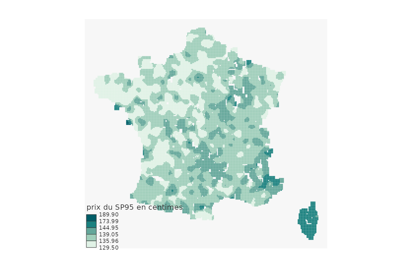
# Example 1
data(dfPrix_SP95_2016)
dfPrix_SP95_2016$nbObs <- 1L
dfSmoothed <- btb::btb_smooth(pts = dfPrix_SP95_2016,
sEPSG = "2154",
iCellSize = 5000L,
iBandwidth = 30000L,
inspire = TRUE)
dfSmoothed$prix95 <- dfSmoothed$SP95 / dfSmoothed$nbObs * 100
library(mapsf)
mf_map(dfSmoothed,
type = "choro",
var = "prix95",
breaks = "fisher",
nbreaks = 5,
border = NA,
leg_title = "prix du SP95 en centimes")
#> Warning: N is large, and some styles will run very slowly; sampling imposed
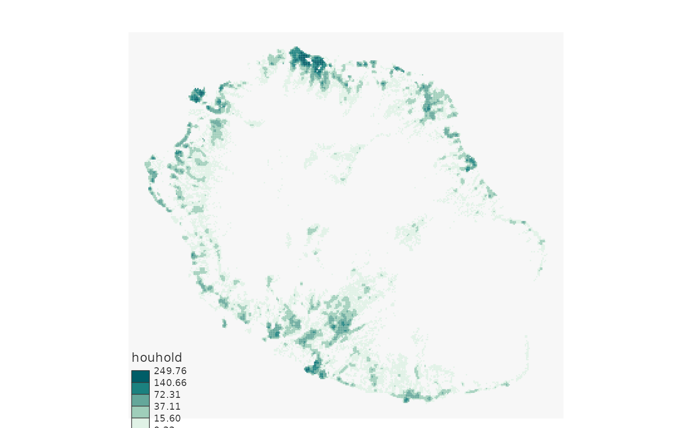
 # Example 2
data(reunion)
# Call mode 1: classic smoothing - automatic grid
reunionSmoothed <- btb_smooth( pts = reunion,
sEPSG = "32740",
iCellSize = 200L,
iBandwidth = 400L)
library(mapsf)
mf_map(reunionSmoothed,
type = "choro",
var = "houhold",
breaks = "fisher",
nbreaks = 5,
border = NA)
#> Warning: N is large, and some styles will run very slowly; sampling imposed
# Example 2
data(reunion)
# Call mode 1: classic smoothing - automatic grid
reunionSmoothed <- btb_smooth( pts = reunion,
sEPSG = "32740",
iCellSize = 200L,
iBandwidth = 400L)
library(mapsf)
mf_map(reunionSmoothed,
type = "choro",
var = "houhold",
breaks = "fisher",
nbreaks = 5,
border = NA)
#> Warning: N is large, and some styles will run very slowly; sampling imposed
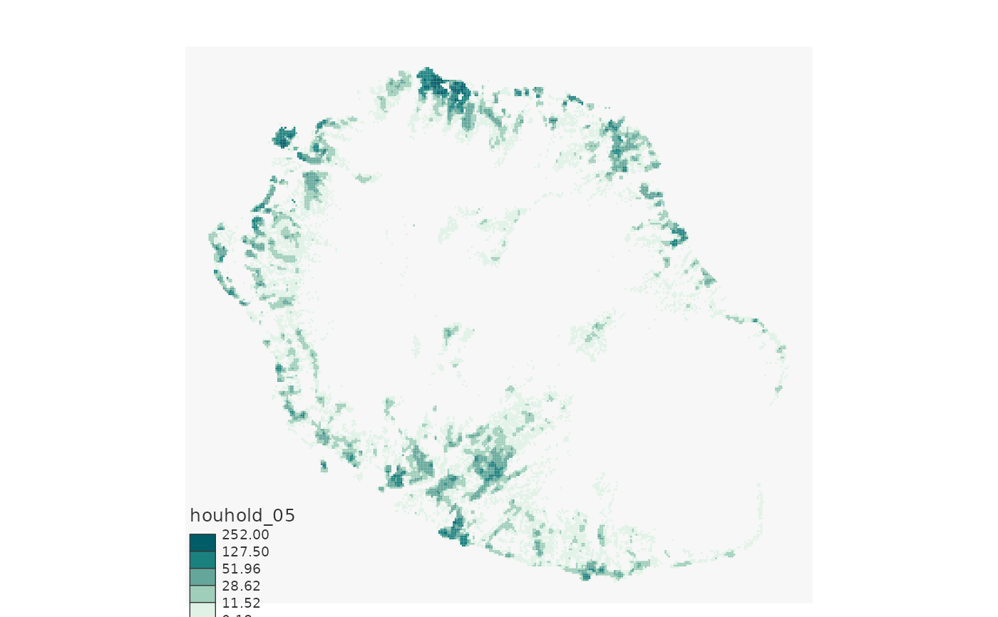
 # Call mode 2: median smoothing - automatic grid
reunionSmoothed <- btb_smooth( pts = reunion,
sEPSG = "32740",
iCellSize = 200L,
iBandwidth = 400L,
vQuantiles = c(0.1, 0.5, 0.9))
mf_map(reunionSmoothed,
type = "choro",
var = "houhold_05",
breaks = "fisher",
nbreaks = 5,
border = NA)
#> Warning: N is large, and some styles will run very slowly; sampling imposed
# Call mode 2: median smoothing - automatic grid
reunionSmoothed <- btb_smooth( pts = reunion,
sEPSG = "32740",
iCellSize = 200L,
iBandwidth = 400L,
vQuantiles = c(0.1, 0.5, 0.9))
mf_map(reunionSmoothed,
type = "choro",
var = "houhold_05",
breaks = "fisher",
nbreaks = 5,
border = NA)
#> Warning: N is large, and some styles will run very slowly; sampling imposed
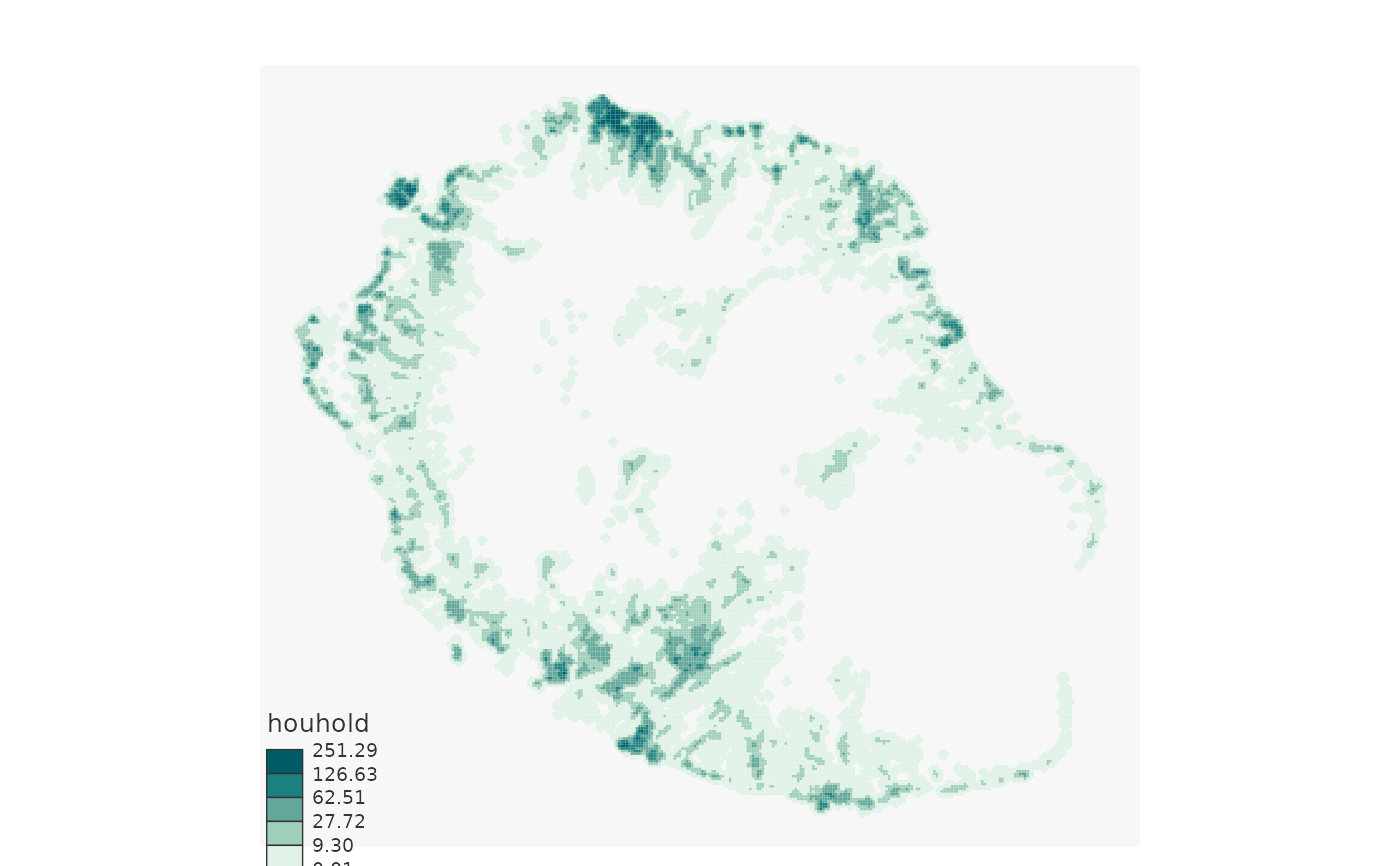
 # Call mode 3: classic smoothing - user grid
dfCentroidsUser <- merge( x = seq(from = 314400L, to = 378800L, by = 200L),
y = seq(from = 7634000L, to = 7691200L, by = 200L))
reunionSmoothed <- btb_smooth( pts = reunion,
sEPSG = "32740",
iCellSize = 200L,
iBandwidth = 400L,
dfCentroids = dfCentroidsUser)
reunionSmoothed <- reunionSmoothed[reunionSmoothed$houhold > 0, ]
mf_map(reunionSmoothed,
type = "choro",
var = "houhold",
breaks = "fisher",
nbreaks = 5,
border = NA)
#> Warning: N is large, and some styles will run very slowly; sampling imposed
# Call mode 3: classic smoothing - user grid
dfCentroidsUser <- merge( x = seq(from = 314400L, to = 378800L, by = 200L),
y = seq(from = 7634000L, to = 7691200L, by = 200L))
reunionSmoothed <- btb_smooth( pts = reunion,
sEPSG = "32740",
iCellSize = 200L,
iBandwidth = 400L,
dfCentroids = dfCentroidsUser)
reunionSmoothed <- reunionSmoothed[reunionSmoothed$houhold > 0, ]
mf_map(reunionSmoothed,
type = "choro",
var = "houhold",
breaks = "fisher",
nbreaks = 5,
border = NA)
#> Warning: N is large, and some styles will run very slowly; sampling imposed
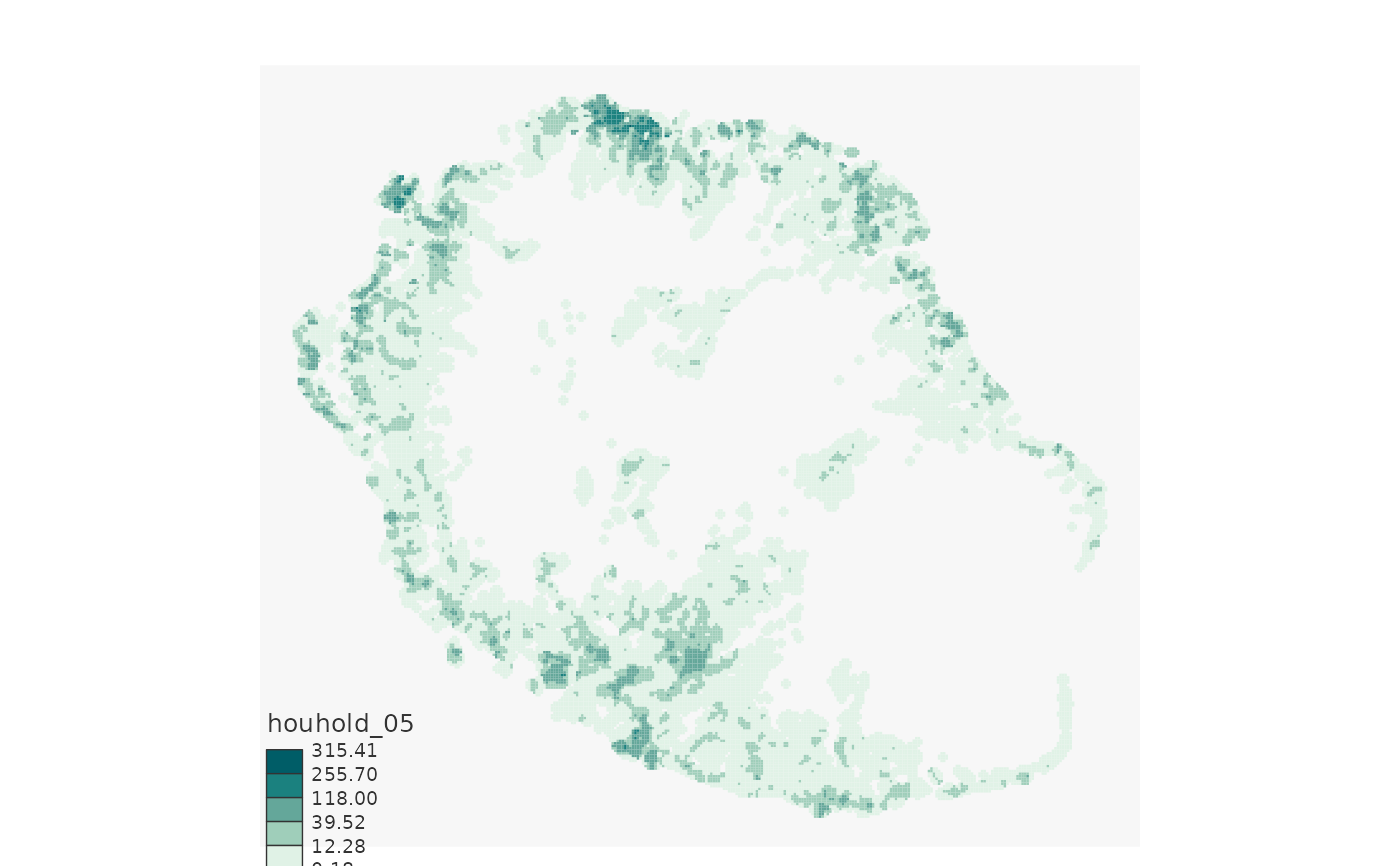
 # Call mode 4: median smoothing - user grid
reunionSmoothed <- btb_smooth( pts = reunion,
sEPSG = "32740",
iCellSize = 200L,
iBandwidth = 400L,
vQuantiles = c(0.1, 0.5, 0.9),
dfCentroids = dfCentroidsUser)
reunionSmoothed <- reunionSmoothed[reunionSmoothed$nbObs > 0, ]
mf_map(reunionSmoothed,
type = "choro",
var = "houhold_05",
breaks = "fisher",
nbreaks = 5,
border = NA)
#> Warning: N is large, and some styles will run very slowly; sampling imposed
# Call mode 4: median smoothing - user grid
reunionSmoothed <- btb_smooth( pts = reunion,
sEPSG = "32740",
iCellSize = 200L,
iBandwidth = 400L,
vQuantiles = c(0.1, 0.5, 0.9),
dfCentroids = dfCentroidsUser)
reunionSmoothed <- reunionSmoothed[reunionSmoothed$nbObs > 0, ]
mf_map(reunionSmoothed,
type = "choro",
var = "houhold_05",
breaks = "fisher",
nbreaks = 5,
border = NA)
#> Warning: N is large, and some styles will run very slowly; sampling imposed
 # }
# }